VRChat Retention, Part 3: When Simple Survival Models Are Not Enough

VRChat Retention — a Bayesian survival analysis of 267,903 VRChat reviewers on Steam (not all players — see Part 1), built entirely from public data. Headline: churn risk collapses in the first 90 days and then goes flat for three years, and the five engagement segments are on genuinely different clocks.

Part 1 — the estimand · Part 2 — three regimes · Part 3 — when simple models fail · Part 4 — five lifecycles · Part 5 — from model to decision

If you are reading for the findings rather than the method, this part is the model-selection argument — skip to Part 4 and Part 5, which is where the users and the decisions are. The one thing worth carrying out of here is in §8.

The short version

Adding five things you know about a user was worth less than getting the timing right — much less. That is the headline, and it decides where modelling effort is worth spending on a retention problem.

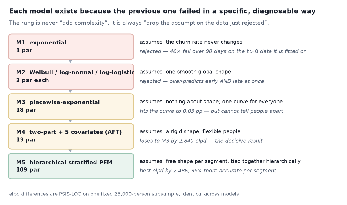
In technical terms: four models, in order, each fitted because the previous one failed in a way I could name. The most informative result in the whole project is not the winner. It is that a model with five covariates lost to a model with none, by a wide margin, because it had the wrong hazard shape. Flexibility in time turned out to matter far more than flexibility in people — and you need to know that before you decide where to spend your modelling effort.

This part also contains a correction I found while writing it.

---

1. The rule

Start with the simplest model that could plausibly explain the data. Add complexity only when the data has rejected the assumption the simpler model was making. Never add a rung because the result would be more impressive.

Each model was fitted because the previous one failed in a specific, diagnosable way.

2. Model 1 — a constant hazard, fitted knowing it would fail

\[h(t) = \lambda, \qquad S(t) = e^{-\lambda t}\]

One parameter for the entire platform: risk on day 1 equals risk on day 1,000. Part 2’s headline 212× is an all-users figure, driven by the day-zero atom; on the t > 0 population these models are actually fitted on, the hazard still falls 46-fold between the first day and day 90. Either way a constant rate is dead on arrival, so this model was fitted precisely because it should lose — a baseline you expect to lose is the only way to know whether later complexity buys anything.

The prior. log λ ~ Normal(−7, 1.5), centred on a median lifetime of about 760 days — the right order of magnitude, deliberately not the 962 days the Kaplan–Meier curve shows, so the data is not used twice. A prior predictive check puts 95% of prior mass on median lifetimes between 41 and 13,952 days, with the observed 962 comfortably interior.

Result. Constant hazard 0.076% per day, implied median 912 days. The like-for-like comparison is the Kaplan–Meier median of the population M1 was actually fitted on — the 245,102 with t > 0, whose median is 1,106 days, not the 962 of the full sample. M1 is 194 days short, not 50. Converged cleanly (R̂ 1.005, ESS 1,416, zero divergences), and the survival curve misses at both ends, exactly as predicted.

3. Model 2 — three smooth shapes, so “which shape?” becomes an empirical question

Weibull, log-normal and log-logistic cost the same two parameters and permit different hazard shapes: Weibull’s is monotone by construction, while the other two can rise then fall. Fitting all three turns a modelling preference into a measurement — and it is worth noting that the fitted log-logistic shape came out at 0.94, below 1, so its hazard is monotone decreasing too. Given the freedom to bend, it declined to.

Priors in business units. For Weibull and log-logistic: log(scale) ~ Normal(7, 1.5) — e⁷ is 1,097 days — and log(shape) ~ Normal(0, 0.5), centred on 1. For the Weibull, shape 1 is the exponential, so centring there means the prior assumes no decay at all. The posterior lands at 0.813, which makes the falling hazard visibly the data speaking rather than the prior. (The log-normal is parameterised differently — mu ~ Normal(7, 2), s ~ HalfNormal(2) — because it has no shape parameter of the same kind.)

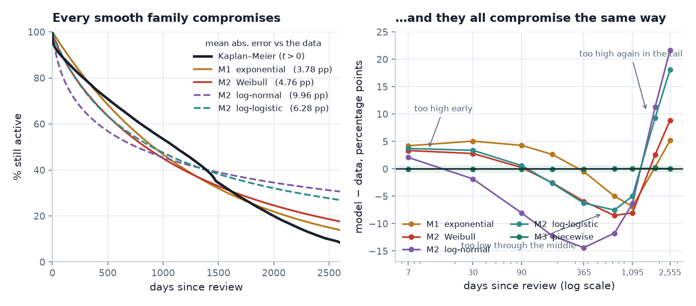Left: fitted survival curves against Kaplan–Meier. Right: signed error at nine horizons. Every smooth family is too high early, too low through the middle, and too high again in the tail.

That error pattern is the signature of a shape mismatch. The families are not badly estimated; they are being asked to make a shape they cannot make, so they compromise, and the compromise is visible as a systematic sign pattern rather than as noise.

A correction, made while writing this series

Models 1 and 2 are fitted on the 245,102 people with t > 0 (Part 1). Their published survival-curve error, however, was measured against the Kaplan–Meier curve of all 267,903 — a curve that sits about 8 points lower early on because it contains the day-zero atom. That compares a conditional survival function against an unconditional one. Model 3’s error was measured correctly, against the t > 0 curve.

Corrected, like-for-like, mean absolute error across the nine published horizons — and, because those nine horizons are all piecewise-exponential knots, where a PEM is exact by construction, the same comparison on a daily grid:

Model	as published	corrected, knot grid	corrected, daily grid
M1 exponential	7.13 pp	3.78 pp	3.63 pp
M2 Weibull	6.27 pp	4.76 pp	5.60 pp
M2 log-logistic	7.69 pp	6.28 pp	7.82 pp
M2 log-normal	8.22 pp	9.96 pp	11.20 pp
M3 piecewise	0.03 pp	0.03 pp	0.22 pp

The knot grid flatters M3 badly: its survival curve passes through the data exactly at its own cut points and bows away in between, so nine-of-nine knots is the one grid on which it cannot lose. On a daily grid its error is 7× larger (worst case 1.23 pp, at day 1,287), and the gap to the best smooth family falls from 132× to 17×.

The conclusion does not move — 17× is still decisive, and the both-ends compromise is still there. Two things do move, and both are worth having. The ranking within the smooth families changes: on the corrected metric the one-parameter exponential tracks the marginal curve better than Weibull, while sitting fifth of seven on out-of-sample predictive score. And the honest statement of M3’s fit is 0.22 pp, not 0.03 pp.

The out-of-sample comparison below is unaffected: PSIS-LOO for every model is computed on the same fixed 25,000-person subsample, drawn with the same seed from the same t > 0 population. For M4 the score is the AFT component only — the hurdle term is not in it — so all seven models are scored on the same conditional density.

4. Model 3 — drop the shape constraint entirely

If no global shape works, stop choosing one. Split the timeline into 18 intervals and let the hazard be constant within each and free between them:

\[h(t) = \lambda_k \quad \text{for } t \in I_k, \qquad k = 1 \dots 18\]

The cut points are not guessed. They are dense where Part 2 measured the hazard moving fastest — 1, 3, 7, 14, 30, 60, 90, 180 days — then half-yearly to two years (365, 547, 730) and yearly after that (1095, 1460, 1825, 2190, 2555), closing with 3000 and 4000. The last three cuts sit beyond Part 2’s descriptive band grid; they exist to give the thin tail somewhere to go, not because the data pointed at them.

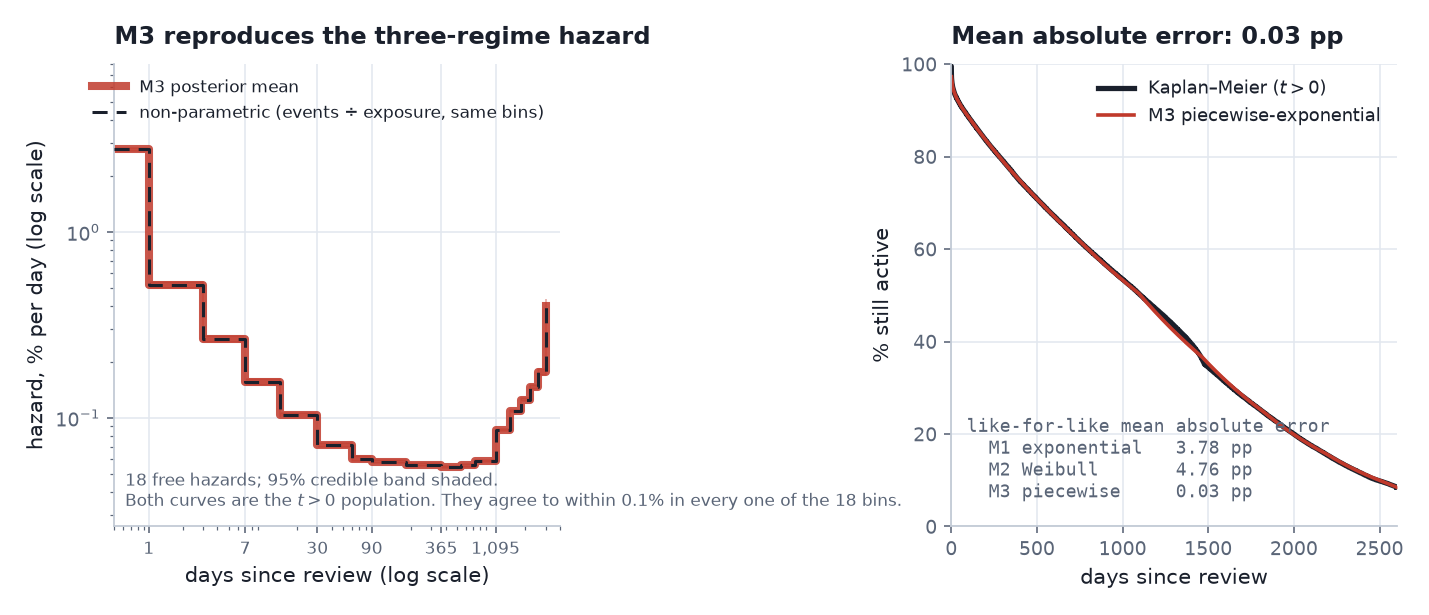Left: 18 free hazards with 95% credible bands, against the raw events-÷-exposure hazard in the same bins and on the same population. Right: the survival fit.

Mean absolute error: 0.22 percentage points on a daily grid (0.03 pp if you only look at the model’s own knots, which is the flattering number and the one I originally published). More convincingly, the posterior mean hazard recovers the raw events-÷-exposure rate to within 0.1% in every one of the 18 bins — a stricter check than the survival curve, because errors in a hazard do not cancel the way errors in a cumulative quantity can. From 5.60 to 0.22 by removing an assumption rather than adding information: M3 has no covariates at all.

Two priors, and why the simpler one is kept

The literature default for a piecewise-exponential hazard is a random-walk smoothing prior on the log-hazard, which borrows strength between neighbouring intervals. Independent weakly-informative priors are the simpler alternative. I fitted both.

They agree to 0.25% at every interval. With 245,102 people the thinnest interval still holds 748 events, so the likelihood pins each hazard down and there is essentially nothing for a smoothing prior to do. The independent version is kept for speed — 2.5 s versus 94.1 s, ESS 11,009 versus 682 — with the note that the random walk would be the correct choice on a sparser dataset.

A correction I had to make to my own diagnosis

An earlier version reported that the random-walk prior was weakly identified, citing R̂ 1.06 and ESS 58, and explained it structurally. That measurement was taken in float32; under float64 the same model with identical settings gives R̂ 1.004, ESS 682. The bad mixing was precision, not statistics. Part 4 §6 has the second and worse instance, with the controlled re-run.

The engineering that makes it fast

For a piecewise-exponential model without covariates, the likelihood reduces exactly to sufficient statistics: events and exposure per interval. That is 36 numbers instead of 245,102 rows.

The naive per-person form does a 245k × 18 matrix multiply inside every leapfrog step. The sufficient-statistic form samples in 2.5 seconds. Because that reduction sits on the critical path of every downstream result, it is tested rather than trusted: it reproduces the per-person log-likelihood to 1e-16. The pointwise log-likelihood needed for PSIS-LOO is reconstructed afterwards from the draws.

Two silent memory bugs are worth recording, because both produced correct numbers and would never have shown up in a result. az.from_numpyro(..., log_likelihood=True) stores one log-density per observation per draw — at 245,102 × 4,000 that is a 7.3 GB posterior for a one-parameter model. And in Model 4 the AFT scale was registered with numpyro.deterministic; it has one value per person, so every draw stored a 245,102-vector — 3.9 GB for a 13-parameter model. The general rule: never register a deterministic whose leading dimension is the sample size.

5. Model 4 — covariates, on a rigid shape

Now the other axis. Part 1 established that 8.5% of people were already gone at the origin, so the model has to be two-part:

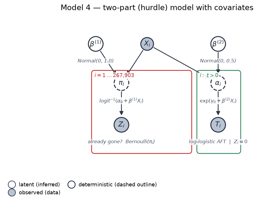Part 1: a logistic model for “already gone at the origin”, on all 267,903. Part 2: a log-logistic AFT for how long the rest last, on the 245,102 with t > 0. Shaded nodes are observed, dashed are deterministic, boxes are plates.

Log-logistic is chosen for the second part over log-normal — the comparison the code actually makes — because it won on predictive score between those two (−151,791 against −154,951) and has the heavier tail, which matters when 26.6% of this sample is censored and therefore lives in that tail. (26.6%, not the 24.3% of the full population: part 2 is fitted on t > 0, and the day-zero atom is all events.)

The obvious cross-question: Weibull beat both on elpd, and Weibull is also an AFT family — why not use it? Because Weibull’s hazard is monotone by construction, and Part 2’s entire finding is that the hazard is not monotone. The fitted log-logistic shape is 1.014, i.e. non-monotone. The deeper answer is that it did not matter: M4 lost to M3 regardless, so the family choice inside M4 was never the binding constraint.

All continuous covariates are standardised so one prior scale is meaningful for all of them. The AFT coefficients get β ~ Normal(0, 0.5) on the log-time scale, which puts 95% of prior mass on lifetime multipliers between 0.38× and 2.66× per standard deviation. The hurdle coefficients get the wider Normal(0, 1), because a log-odds scale needs more room than a log-time scale. Both regularise without deciding the answer.

The coefficients are genuinely useful, and they are the reason M4 survives into the final write-up at all:

Covariate	Lifetime multiplier, per SD	95% CrI
log playtime at review	×2.11	[2.09, 2.13]
games owned on Steam	×1.30	[1.29, 1.31]
public profile	×1.12	[1.11, 1.13]
recommended the game	×1.10	[1.09, 1.11]
reviewed in English	×1.05	[1.05, 1.06]

And for the hurdle — the odds of having already left before writing the review:

Covariate	Odds ratio
log playtime at review	0.18
recommended the game	0.57
reviewed in English	0.84

Playtime dominates both halves, and nothing else is close.

6. The result that matters most

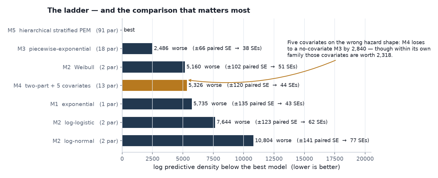PSIS-LOO expected log predictive density, relative to the best model. Standard errors are paired — see below.

Model	Params	elpd	vs best
M5 hierarchical stratified PEM	91 †	−144,148	—
M3 piecewise-exponential	18 †	−146,634	−2,486
M2 Weibull	2	−149,307	−5,160
M4 two-part + 5 covariates	13	−149,474	−5,326
M1 exponential	1	−149,882	−5,735
M2 log-logistic	2	−151,791	−7,644
M2 log-normal	2	−154,951	−10,804

† Sampled free parameters. The project’s own result table records M3 as 19 (counting the discarded random-walk parameterisation: an intercept, a scale and 17 increments) and M5 as 109 (counting the 90 deterministic cell hazards on top of the 19 hyperparameters that generate them). The models actually fitted sample 18 and 91. I flag it because both sets of numbers appear in the same repository and someone will notice.

Model 4 loses to Model 3 by 2,840 elpd, despite having five covariates that Model 3 does not have. It also loses to a two-parameter Weibull with no covariates (by 166) and beats a one-parameter constant hazard by only 409.

There are two honest ways to read that, and both belong in the write-up:

• Within its own family, covariates are worth 2,318 elpd — log-logistic with them against log-logistic without. Covariates work.
• Across families, the shape choice dominates them completely.

Reporting only the first would be flattering and misleading. What the pair says together is: for this dataset, get the time structure right before you get the people structure right. If I had started with a covariate model — the instinct most of us have — I would have spent the effort on the axis that mattered less, and the fit statistics would have looked respectable enough that I might never have noticed.

The standard errors were wrong in the safe direction

The original comparison used se = √(se_A² + se_B²), which assumes the two models’ errors are independent. They are not — every model is scored on the same 25,000 people. The correct paired standard error is √n · sd(pointwise differences).

One labelling correction while I am here: the paired numbers below are computed on the in-sample pointwise log predictive density, not on PSIS-LOO — the script differences logsumexp values with no importance weighting. Running PSIS properly gives 2,500.3 ± 65.6, i.e. 38.1 standard errors instead of 38.0, so nothing moves. But calling an lppd difference a PSIS-LOO difference is exactly the sloppiness this post spends a table correcting elsewhere:

Comparison	naive SE	paired SE	naive verdict	paired verdict
M5 vs M3	713	66	3.5 SEs	38.0 SEs
M5 vs M2 Weibull	718	102	7.2 SEs	50.9 SEs
M5 vs M2 log-normal	746	141	14.5 SEs	76.9 SEs

Every comparison was already decisive and is now overwhelmingly so. No conclusion changes — but the naive form was the kind of error that changes conclusions in a closer race, so it is worth fixing when it doesn’t.

7. Where that leaves the model

M3 has the time structure and no way to tell people apart. M4 can tell people apart and has the wrong time structure. Part 2 measured a 3.9× spread between segments, so ignoring people is not an option either.

The requirement is now precise: a hazard free to vary over time, and free to vary differently for different kinds of user, without letting the sparse corners of that grid produce nonsense.

8. What this means for a data team

This part has no customer-facing finding in it. It has a resourcing one, and it is the most transferable thing in the series.

Get the time structure right before you add features. Five covariates fitted onto the wrong hazard shape lost to a model with no covariates at all, and lost to a two-parameter model with no covariates. If you have one week on a retention problem, the evidence here says spend it on the shape of the hazard, not on feature engineering. The instinct most teams have — start with a covariate model, iterate on features — would have spent the week on the axis that mattered less, and the fit statistics would have looked respectable enough that nobody noticed.

Model choice has an infrastructure cost, and it is not the one you expect. The piecewise-exponential likelihood reduces exactly to 36 numbers, so the fit is independent of sample size — 2.5 seconds on 245,102 people. The same model written naively does a 245k × 18 matrix multiply inside every leapfrog step. That is the difference between a model you can re-run on every data refresh and one you run once and never touch. The reduction is verified to 1e-16 precisely because so much rests on it.

Never register a deterministic whose leading dimension is the sample size. Two silent memory bugs in this project produced perfectly correct numbers while writing multi-gigabyte posteriors — 7.3 GB for a one-parameter model. Nothing in any result would ever have shown it.

And the meta-point: every rung of this ladder is a model I expected to lose, fitted so that the next one had something to beat. The failures are the deliverable. A progression that jumps straight to the hierarchical model produces identical final numbers and no way to defend them.

Next: Part 4 — beyond the average user. The final model, why it is not a proportional-hazards model in disguise, and the convergence failure I spent real effort explaining statistically before discovering it was a floating-point default.